Analysis | |
| Prev | Knots and Links | Next |
You can view a variety of information about the link diagram, as well as topological invariants of the link itself, by stepping through the different tabs in the link viewer. Here we talk through the different kinds of information and invariants on offer.
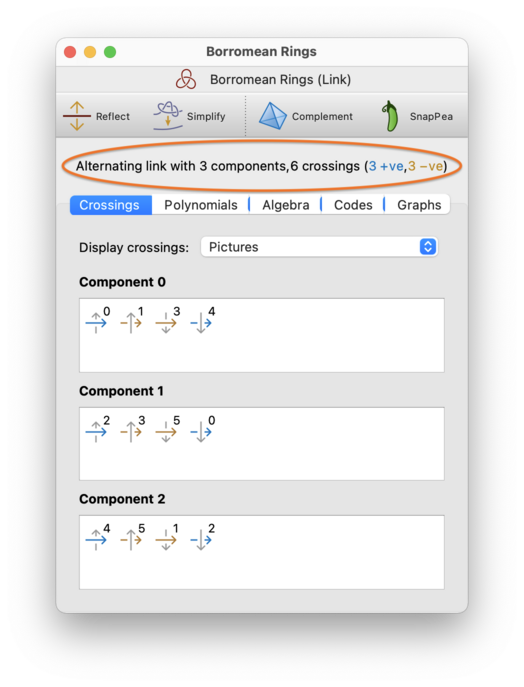
At the top of each link viewer is a header, which includes: whether the link is alternating; the number of link components (or the word “knot” to indicate just one); and the number of crossings, including how many are positive and negative.
This header is circled in red below.
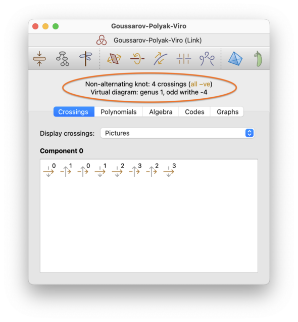
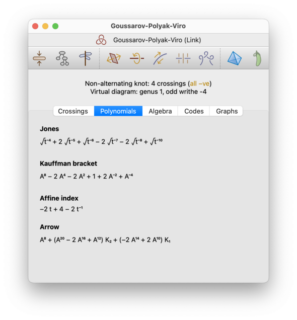
If the link diagram is virtual (not classical), then the header will contain a second line indicating:
The virtual genus of the diagram. This is the smallest genus of orientable surface in which the diagram embeds. Note that this is a property of the link diagram, not an invariant of the link itself.
The odd writhe, or self-linking number. This is an invariant of virtual knots (but not links), which sums the signs of all odd crossings. A crossing
cis odd if, when traversing the knot, we pass through an odd number of crossings between the over-strand and the under-strand ofc.The odd writhe is not shown for multiple-component links. For classical knots, the odd writhe is always zero.
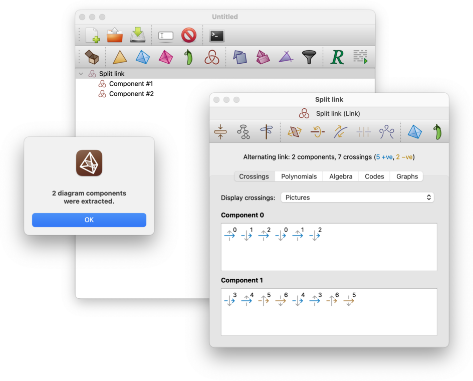
The Crossings tab shows the details of the individual crossings and components that make up the link. Regina numbers crossings 0,1,2,…, and likewise for components.
For each component of the link, there will be a box beneath the Crossings tab showing the crossings that you visit in order as you traverse the link component from an arbitrary starting point. There are two different ways that you can view this information (with a drop-down box to switch between them):
- Pictures
Each crossing will be shown visually as a pair of arrows, one crossing over the other. One arrow will be a solid colour, and will run horizontally from left to right; this is the part of the link that you are traversing. The other arrow will be grey, and will run vertically (either up or down); this is the part of the link that you are passing over or under. The crossing number will be written in the top-right corner beside the arrows.
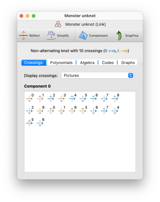
For each crossing, the arrow that you are traversing will be coloured blue for a positive crossing, or yellow for a negative crossing. (This is just a visual aid, and is not strictly necessary; you can already tell the sign of the crossing from the arrangement of the arrows.)
Crossings are visited in order from left to right along each row of the display, one row at a time (i.e., the same way that you would read English text in a book).
Tip
Because the arrows you traverse always run from left to right, you can imagine the individual crossings as being attached together in the order that they are displayed. In other words, you can picture the link component as a long arrow running from left to right through the individual crossings (and then wrapping around to the next line each time it reaches the right-hand edge of the window). Of course this picture breaks down once you revisit the same crossing for a second time.
- Text
Each crossing will be shown as a number with a plus or minus sign attached. The number indicates which crossing you are passing through, and the sign indicates whether it is a positive or negative crossing. The sign will appear as a superscript if you are passing over the crossing, or a subscript if you are passing under.
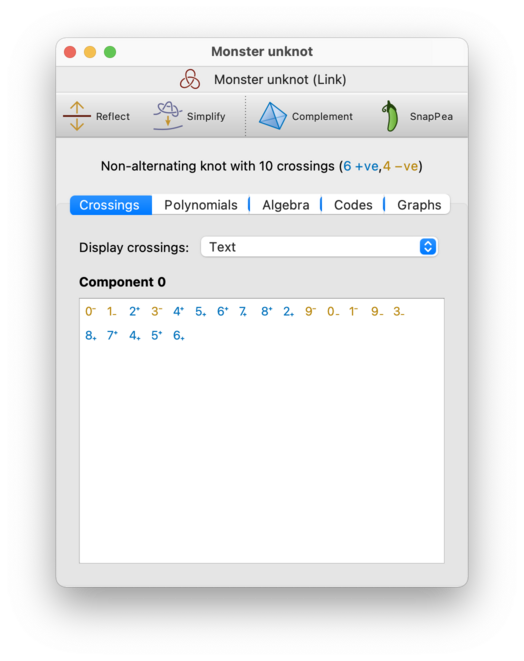
As before, crossings are visited in order from left to right along each row, one row at a time. Also as before, positive crossings will be coloured blue and negative crossings will be coloured yellow (but again the colour is just a visual aid, since you already have this information from the plus/minus sign).
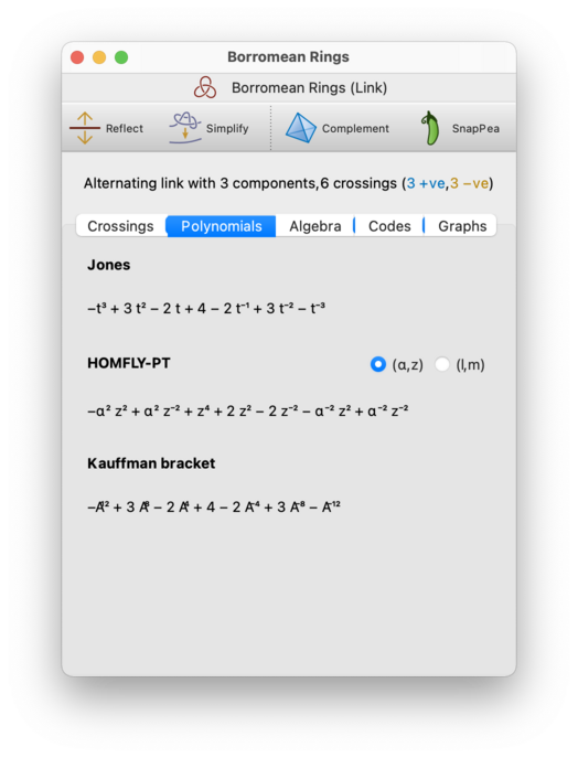
On the Polynomials tab, you can view several polynomial invariants of the link and of the link diagram. Which polynomials you see will depend upon whether your link diagram is classical or virtual.
The polynomials that you might see include:
- Alexander (classical only)
The Alexander polynomial is a single-variable polynomial invariant. It is relatively weak, but (unlike many of the other invariants listed here) it can be computed in polynomial time.
Regina will only compute Alexander polynomials for knots (not multiple-component links).
- Jones (classical and virtual)
The Jones polynomial is a single-variable polynomial in the variable
t, whose exponents are integers for classical knots, but whose exponents may be half-integers in other cases (depending on the number of link components and/or whether the link is virtual). You may therefore see this presented either as a polynomial intor as a polynomial in √t.If you have opted not to use unicode symbols, then you will see this as a polynomial in either
torsqrt_t.Regina can compute Jones polynomials for link diagrams with any number of components.
- HOMFLY-PT (classical only)
The HOMFLY-PT polynomial is a two-variable polynomial with two common formulations: one in the variables (
α,z) and one in the variables (l,m). These formulations give different polynomials, which are related via a simple substitution. Regina offers a pair of buttons beside the HOMFLY-PT polynomial for you to choose which formulation is displayed.Regina can compute HOMFLY-PT polynomials for link diagrams with any number of components.
- Kauffman bracket (classical and virtual)
The Kauffman bracket is a property of the link diagram, not an invariant of the link, and is related to the Jones polynomial by a simple substitution. See Adams [Ada94] for a simple combinatorial introduction to the Kauffman bracket and the Jones polynomial.
Regina can compute Kauffman brackets for link diagrams with any number of components.
- Affine index (virtual only)
The affine index polynomial is a single-variable polynomial invariant that is relatively weak, but which nevertheless provides some useful information for virtual knots. Its main advantage is that it is extremey fast to compute even for large knot diagrams (the computation runs in very small polynomial time).
Regina will only compute affine index polynomials for virtual knots (not multiple-component virtual links).
The affine index polynomial is not shown at all for classical link diagrams, since in the classical case the affine index polynomial is always zero.
- Arrow (virtual only)
The arrow polynomial enhances the Kauffman bracket in a way that makes it more powerful for virtual links, and that makes it a true link invariant. Whereas the Kauffman bracket is a polynomial in the single variable
A, the arrow polynomial is a polynomial in many variables (A,K1,K2,K3, …).Regina can compute arrow polynomials for virtual link diagrams with any number of components.
The arrow polynomial is not shown at all for classical link diagrams, since in the classical case the arrow polynomial is just the Kauffman bracket with some normalisation applied.
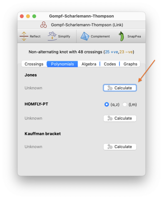
For larger links, you may see a Calculate button instead of a polynomial. This is because many of these polynomials require exponential time to compute. In this case you will need to press the Calculate button and be prepared to wait—for most polynomials you will see the progress displayed, and you can cancel the computation if you like.
For smaller links, all of the polynomials will be computed automatically.
Tip
You can copy any of these polynomials to the clipboard by right-clicking and selecting either Copy or Copy plain text. If you press Copy then the polynomial will be copied using unicode symbols, and if you press Copy plain text then the polynomial will be copied in plain ASCII symbols using a simple “pidgin TeX”.
Tip
If you find the polynomial exponents hard to read (due to the subscripts being very small), you can visit Regina's settings and disable unicode symbols. This will change the polynomial display to use a simple “pidgin TeX” instead.
The Algebra tab holds several smaller tabs that describe different groups associated with the link.
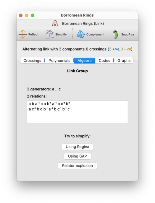
Currently this shows the following groups:
- Knot/Link Group
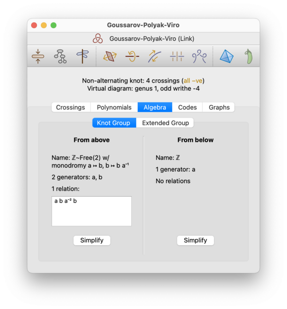
This is the link group as constructed from the Wirtinger presentation (though Regina will typically simplify the presentation before showing it here). Each relation is some variant of the form
xy=yz, whereycorresponds to the upper strand at some crossing, andxandzcorrespond to the two sides of the lower strand at that same crossing.For classical links, this is isomorphic to the fundamental group of the link complement. However, it is constructed differently, and so it may have a different presentation. If you are having difficulty simplifying it, you could perhaps try working with the triangulated link complement instead.
For virtual links, the link group could change depending upon whether you view the link from above or below the diagram (i.e., rotating the link may change the isomorphism class). For this reason, if the link diagram is virtual then you will see two groups: one as seen from above (using the classical Wirtinger presentation), and one as seen from below (obtained by switching the upper and lower strands at every crossing). The Goussarov-Polyak-Viro knot (which is one of Regina's ready-made examples is a nice example of where these two groups differ.
Note however that, for virtual links, the link group is not a particularly strong invariant. You might wish to work with the extended group instead (see below).
- Extended Group
This is the extended group of the link, as defined by Silver and Williams [SW06]. This invariant is particularly useful for virtual links, where the ordinary link group is a fairly weak invariant. However, it also yields more complex group presentations.
Like the ordinary link group, the extended group of a virtual link may change depending upon whether you view the link from above or below the diagram, and so for virtual link diagrams Regina will display both variants.
All groups will be presented in the same format as the fundamental group of a triangulation, and you are given the same tools to simplify them. See the section on fundamental groups for further discussion of this.
Tip
If you find the exponents in the group presentations hard to read (due to the superscripts being very small), you can visit Regina's settings and disable unicode symbols. This will change the display to use a simple “pidgin TeX” instead.
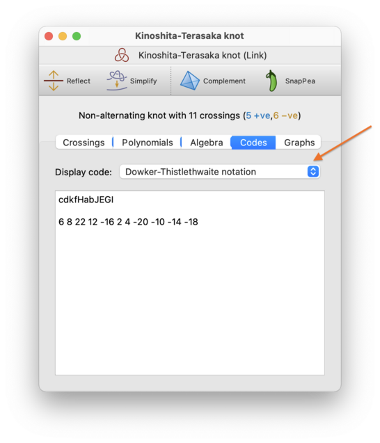
The Text Codes tab allows you to export your knot or link in several text-based formats. Simply select a format from the drop-down box (indicated in the screenshot below), and the corresponding text code will be shown in the box beneath.
The codes that Regina can display include:
- Gauss codes
This displays the classical, oriented and signed Gauss codes. Classical Gauss codes are common in the literature, but they suffer from ambiguities related to orientation; for composite knots they may not even uniquely define the topology. Oriented and signed Gauss codes solve this problem by adding a little more information.
For a more detailed description of these formats, see the section on creating knots from Gauss codes.
Currently Regina only displays Gauss codes for knots (not multiple component links). If your knot diagram is virtual (not classical), then Regina will still display all three Gauss codes; however, only the oriented and signed variants contain enough informtion to reconstruct the diagram.
- Dowker-Thistlethwaite notation
Like classical Gauss codes, Dowker-Thistlethwaite notation is also common in the literature, and also suffers from ambiguities related to orientation and composite knots. Dowker-Thistlethwaite notation comes in two forms—numerical and alphabetical—and Regina displays both forms here.
For a more detailed discussion of Dowker-Thistlethwaite notation, see the section on creating knots from Dowker-Thistlethwaite notation.
Currently Regina only displays Dowker-Thistlethwaite notation for knots (not multiple component links), and only for classical (not virtual) knot diagrams. Be aware that alphabetical Dowker-Thistlethwaite notation is case-sensitive (i.e., upper-case and lower-case matters).
- Knot/link signature
Knot/link signatures are Reginas own text-based format, and were designed to have a combinatorial uniqueness property: two link diagrams have the same signature if and only if they are combinatorially isomorphic (which includes relabelling crossings and/or components, reflecting the entire diagram, rotating the entire diagram, and/or reversing individual link components).
For a more detailed discussion of knot/link signatures, see the section on creating knots from knot/link signatures.
These signatures are supported for all links with fewer than 64 components, and they support both classical and virtual link diagrams. Be aware that knot/link signatures are case-sensitive (i.e., upper-case and lower-case matters).
- Planar diagram codes
This displays the planar diagram code for the link. Planar diagram codes support multiple-component links, as well as both classical and virtual link diagrams. Their main limitations are that they cannot represent zero-crossing unknot components, and they cannot fix the orientation of a link component that consists entirely of over-crossings.
For a detailed description of planar diagram codes, see the section on creating links from planar diagram codes.
- Jenkins format
This is a multiline text code described by Bob Jenkins, and used in his HOMFLY-PT polynomial software. Regina can happily display the Jenkins format for multiple-component links, and for both classical and virtual link diagrams.
In this format, a link is described by a sequence of integers separated by whitespace. We assume that there are
ncrossings in the link, labelled arbitrarily as 0,1,2,…. The sequence of integers will contain, in order:the number of components in the link;
for each link component:
the number of times you pass a crossing when traversing the component (i.e., the length of the component);
for each link component: two integers for each crossing that you pass in such a traversal: the crossing label, and then either +1 or -1 according to whether you pass over or under the crossing respectively;
for each crossing:
the crossing label;
the sign of the crossing (either +1 or -1).
For all of these text codes except for Jenkins format, you can convert a text code back into a link as described in creating a new link. Be aware that the resulting link might not use the same crossing numbers, and might even be a reflection and/or reversal of the original.
For Jenkins format, Regina's graphical user interface does not offer a
way to convert a code back into a link; however, you can always bring up
a Python console and call the
function Link::fromJenkins() instead.
On the Graphs tab, you can view different graphs associated with the link diagram. These graphs are all related to the diagram graph, which is a 4-valent graph with one vertex for each crossing and edges that follow the strands of the link.
There is a drop-down box for you to choose which graph you want to see. The options are:
- Tree decomposition
A tree decomposition (illustrated below) models the diagram graph using a rooted tree; you can read more about tree decompositions in the triangulations chapter. Regina uses these tree decompositions in its fixed-parameter tractable algorithms for the Jones and HOMFLY-PT polynomials [Bur18].
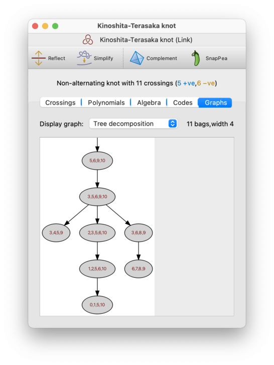
Regina will display both the width and the number of bags above the tree decomposition itself.
As with triangulations, Regina does not guarantee to find a tree decomposition of the smallest possible width (i.e., it does not compute the precise treewidth of the diagram graph). Instead it uses fast heuristics that are found to produce low-width tree decompositions in practice.
- Nice tree decomposition
This is a variant of the tree decomposition that is less concise, but more useful in practice for algorithms since it imposes very tight constraints on the relationships between parent and child bags. Again, you can read more about these in the triangulations chapter.
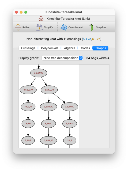
As with tree decompositions, Regina will display both the width of the nice tree decomposition and the number of bags that it contains. Typically the width will be the same as for the (plain) tree decomposition above, but the number of bags may be significantly larger (though still linear in the overall number of crossings).
Regina includes many tools for working with 3-manifold triangulations, as well as working directly with knots and links. If you want access to these 3-manifold tools, you can build a triangulation of the link complement.
The meaning of “complement” in this setting depends upon whether you are working with a classical or virtual link diagram.
If you have a classical link diagram, then Regina will build an ideal 3-manifold triangulation representing the complement of your link in the 3-sphere.
The resulting triangulation will have exactly one ideal vertex for each link component.
If your link diagram is disconnected (in the graph-theoretical sense), then the resulting 3-manifold will be the connected sum of the complements of each connected diagram component. In particular, the resulting triangulation will always be connected.
For classical links, the complement is a topological invariant of the link.
If you have a virtual (non-classical) link diagram, let
Sbe the smallest genus closed orientable surface in which the diagram embeds (this corresponds to the virtual genus of the diagram). Then Regina will build the complement of your link diagram in the thickened surfaceS× I.The resulting triangulation will have one ideal vertex for each link component, plus an additional two ideal vertices for the two copies of
Son the boundary ofS× I.If your link diagram is disconnected (in the graph-theoretical sense), then the surface
Sthat is used will be the connected sum of the individual closed orientable surfaces that host each connected diagram component. In particular, as in the classical case, the resulting triangulation will always be connected.For virtual links, the complement (and indeed the genus of the surface
S) is not a topological invariant, but instead depends upon the specific link diagram.
There are two ways you can build a link complement:
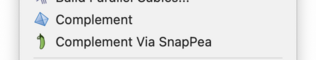
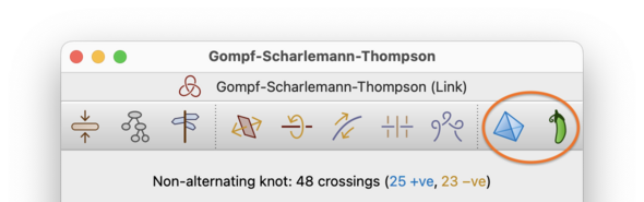
If you select → from the menu or press the corresponding toolbar button (the first button circled above), then Regina will use its own implementation to create a native Regina triangulation of the complement. The triangulation will have access to the full suite of Regina's tools for triangulations, but the meridian and longitude curves from the diagram will be forgotten.
The Complement option is available for all link diagrams, both classical and virtual.
If you select → from the menu or press the corresponding toolbar button (the second button circled above), then Regina will pass the link to the SnapPea kernel to triangulate instead; the result will be a hybrid SnapPea triangulation. The peripheral curves from the diagram will be preserved in SnapPea's data structures; however, the available tools for working with the triangulation combinatorially will be more limited. See the introduction to the chapter on SnapPea triangulations for more information on these limitations.
The Complement Via SnapPea option is only available for classical link diagrams, not virtual diagrams.
Regardless of which method you use, the new triangulation will be inserted immediately beneath your link in the packet tree.
At present Regina only offers very basic algorithms for decomposing links into smaller pieces. These include the following:
If you have a link diagram that is a disjoint union of several smaller diagrams, you can split the diagram into its connected components. Here connected means that you can travel between any two parts of the diagram by following the link and/or jumping between upper and lower strands at crossings. In other words, connectivity refers to the underlying 4-valent graph, where every crossing becomes a 4-way intersection.
What this means:
A disconnected link diagram must describe a splittable link.
A splittable link, however, could be described by a single connected diagram component. For example, you could perform trivial type II Reidemeister moves to make the different link components overlap (thus making the entire link diagram connected).
In general, a single diagram component could contain multiple link components.
To split a link diagram into its connected components, select → from the menu. You must open the link for viewing before you can do this.

Regina will create several new links, one for each connected component of the original diagram. These will be added beneath the original in the packet tree. Your original (disconnected) link diagram will remain unchanged.
| Prev | Contents | Next |
| Knots and Links | Up | Modification |